Gaussian Distribution is All you need
Gaussian Distribution, one of the most important and widely used probability distributions in statistics and machine learning. It is also known as the normal distribution, which is a continuous probability distribution that is symmetric about the mean, showing that data near the mean are more frequent in occurrence than data far from the mean. In the blog, I will walk through the AI field from basic normal distribution, and see how this tree spread across the world.
| Terminology | Description |
|---|---|
| Name | This is hte name |
Definitation of Normal Distribution
Gaussian Distribution
Gaussian distribution, also know as the Normal Distribution, is defined, for a single real-valued variable \(x\) as:
\[ \mathcal{N}(x | \mu, \sigma^2) = \frac{1}{(2\pi\sigma^2)^{1/2}}\exp\left\{- \frac{1}{2\sigma^2} (x - \mu)^2\right\} \tag{1}\]
where:
- \(\mu\) called the mean
- \(\sigma^2\) called the variance
- \(\sigma\) called the standard deviation
- \(\beta = 1/\sigma^2\) called the precision.
Multivariate Gaussian Distribution
Now, we consider the \(D\)-dimensional \(\mathbf{x}\), this lead to the Multivariate Gaussian, which is defined as:
\[ \mathcal{N}(\mathcal{\mathbf{x}|\boldsymbol{\mu}, \boldsymbol{\Sigma}})= \frac{1}{(2\pi)^{D / 2}|\boldsymbol{\Sigma}|^{1 / 2}} \exp\left\{ - \frac{1}{2} (\mathbf{x}- \mathbf{\mu})^{T} \boldsymbol{\Sigma}^{-1}(\mathbf{x} - \boldsymbol{\mu})\right\} \tag{2}\]
where:
- \(\boldsymbol{\mu}\) is the \(D\)-dimensional mean vector
- \(\boldsymbol{\Sigma}\) is the \(D \times D\) covariance matrix - \(\det \boldsymbol{\Sigma}\) is the determinant of \(\boldsymbol{\Sigma}\)
- \(\Lambda \equiv \boldsymbol{\Sigma}^{-1}\) is the precision matrix.
Mixture of Gaussian
More complexity, when we take the linear combination of the basic distribution of Normal Distribution, we will get Mixture of Gaussian Distribution, which is defined as:
\[ p(\mathbf{x}) = \sum_{k=1}^{K}\pi_{k}\mathcal{N}(\mathbf{x} | \boldsymbol{\mu}_{k}, \boldsymbol{\Sigma}_{k}) \tag{3}\]
where:
\(\pi_k\) called the mixing coefficients, who has constraints that
\[ \begin{array} &\sum_{k=1}^K \pi_k = 1 \\ 0 \leq \pi_{k} \leq 1\end{array} \]
\(\mathcal{N}(\mathbf{x} | \boldsymbol{\mu}{k}, \boldsymbol{\Sigma}{k})\) is called a component of the mixture, has its own \(\boldsymbol{\mu}\) and \(\boldsymbol{\Sigma}_k\)
Conditional Distribution
The conditional distribution is defined as
\[ p(\mathrm{x} | \mathrm{y}) \]
which mean the probability distribution function of \(\mathrm{x}\) is dependent on the value of \(\mathrm{y}\). One of the nice property of Gaussian Distribution is that:
If the joint distribution of the two random variable are gaussian distribution, then the conditional distribution is also a Gaussian distribution.
Marginal Distribution
The marginal distribution is defined as:
\[ p(\mathrm{x})= \int p(\mathrm{x}, \mathrm{y}) d\mathrm{y} \]
Another good property of the normal distribution is that:
If the joint distribution of the two random variable are gaussian distribution, then the marginal distribution is also gaussian.
Linear Gaussian Model
Gaussian In High-Dimension
Learning Parameters
From now on, we assume all the \(\mathbf{x}\) are \(D\)-dimensional, as in Equation 2. Because we live in the high-dimensional word.
We have defined three different distributions that has Normal Distribution. The problem is that: how to learn the parameters in the distributions, such as \(\mu\) and \(\sigma\)? Such task is known as Density Estimation.
It should be emphasized that the problem of density estimation is fundamentally ill-posed, because there are infinitely many probability distributions that could have given rise to the observed finite data set.
Pattern Recognition and Machine Learning
How to learn the parameters when all we have the dataset \(\mathcal{D} = {\mathbf{x}_1, \dots, \mathbf{x}_n}\) that has \(N\) data points?
Maximum Likelihood Learning
The first methods we introduce is the maximum likelihood learning, which is defined as:
\[ \max P(\mathcal{D} | \mu, \Sigma) \tag{4}\]
The \(P(\mathcal{D} | \mu, \Sigma)\) is called the likelihood of the dataset, as we defined in the question, the data points are i.i.d. so, we can write the likelihood function as:
\[ P(\mathcal{D} | \mu, \Sigma) = \prod_{n = 1}^N \mathcal{N}(\mathbf{x}_n | \mu, \Sigma) \tag{5}\]
In the practice, because the \(0 \leq \mathcal{N}(\mathbf{x}_n | \mu, \Sigma) \leq 1\), when multiplying \(N\) small number together, might cause the under-flow problem in the computer. So, we use \(\log\)-form of the function to prevent the under-flow. Because the \(\log\) function is the monomtic function, so, when we maximimzie \(\log f\) is same as \(\max f\).
So, the objective function we want to maximize is:
\[ \ln P(\mathcal{D} | \mu, \Sigma) = \sum_{n = 1}^N \ln\mathcal{N}(\mathbf{x}_n | \mu, \Sigma) \tag{6}\]
How to maximize the Equation 6. The most intuitive of way is set the derivative of the function with respect to 0.
Gradient Descent
Bias of Maximum Likelihood Learning.
As we can see, we used the sample mean to derive the sample variance. Because the sample mean estimated from the dataset \(\mathcal{D}\) , it is not same as the true \(\mu\).
Maxium A Posterior(MAP) Estimate
Expectation-Maximization(EM) Algorithms
EM Algorithms for Gaussian Mxiture Model
Sequential Estimation
So far we have assume that we can “see” the whole dataset at once. In practice, we sometime cannot get the whole dataset at one, because:
- The data points comes in sequential, e.g. Online Learning
- The dataset is too big that can not fit into the memory of the computer.
We have to way to learn the parameters in sequential version. One of the method is called Robbins-Monro algorithm.
Welford’s Algorithm
Robbins-Monro Algorithm
Kalman Filter
Stochastic Gradient Descent
Expoential Moving Average(EMA)
Applications
Kernl Density Estimation
Linear Regression
Gaussian Process
Clustering
Deep Learning
Model Initilization
As mention in the (He et al. 2015)
LoRA
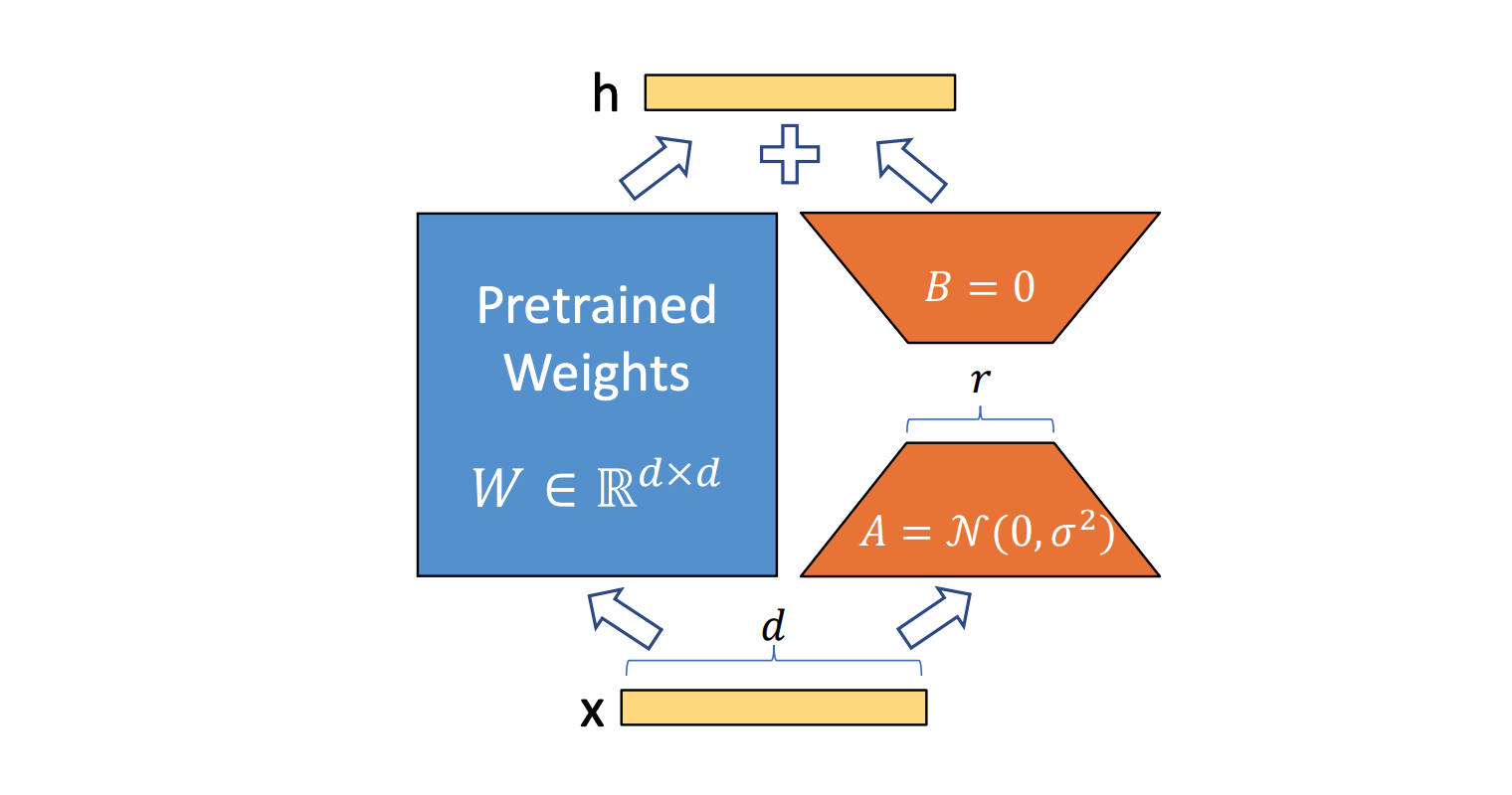
In the LLM, the number of parameters is huge, how we can file-tune those huge parameters. Using parameters efficient fine-tuning technique is one technique. LoRA is one of the PEFT that widely used in the file-tuning huge data.
The \(A\) matrix is initilization as the Normal DistributionEquation 2
Normalization
Layer Normlization
RMS Normlization
This is the RMS with (zhang?)
Generative Models
In the Generative Models, the Normal Distribution is sometime used as the noise add to the original data, or the prior distribution of some unknown distribution that we are trying to get. In this chapter,
Generative Adversarial Networks
The Latent Space input to the generator is of sampled from a Gaussian Distribution (Goodfellow et al. 2014)
Variational Autoencoders(VAE)
VAEs uses a Gaussian Latent space to learn a generative model of data. (Kingma and Welling 2022)
A VAE assumes that data is generated from a latent variable \(Z\), which follows a Gaussian prior: \(Z \sim \mathcal{N}(0, I)\). The VAE model learn a probabilistic mapping from \(Z\) to the observed data \(X\) using:
- Encoder: \(q(Z |X ) \sim \mathcal{N}(\mu_\theta(X), \sigma^2_\theta(X))\)
- Decoder: \(P(X | Z)\) reconstructs \(X\) from \(Z\)
Diffusion Models
(For more details, check my this blog about diffusion models)
This paper (ho?)
Reinforcement Learning
In the Reinforcement Learning, Gaussian Distribution are commonly used in policy gradient methods like Trust Region Optimization(TRPO) and Proximal Policy Optimization(PPO), where policies are modeled as Gaussian distribution.
When Exploration the environment, the exploration is often handled by Gaussian noise, such as in Deep Deterministc Policy Gradient
Meta Learning
Bayesian Meta Learning: Gaussian priors over parameters enable fast adaptation to new tasks in few-shot learning.
Latent Task Representation: Many meta-learning frameworks use Gaussian distributions in the latent space to generalize across different tasks efficiently
Uncertainty Estimation: Gaussian-based models in meta-learning help quantify uncertainty, improving robustness in real-world application.